Quality control

A cell can be bad, the image it came from can be bad, or the whole well can be. This page flags each level on the 13,578 cells of jump_cells(): 24 wells of the JUMP plate BR00121438, four fields of view each, as CellProfiler measured them [Chandrasekaran et al., 2023]. The first call downloads about 1.5 GB.

The QC functions only write flags. The filter_ functions drop what was flagged, and you choose which to call.

import matplotlib.pyplot as plt
import numpy as np
import pandas as pd

import mantispy as mt

cells = mt.ds.jump_cells()
cells

AnnData object with n_obs × n_vars = 13578 × 5839
    obs: 'Metadata_ImageNumber', 'Metadata_ObjectNumber', 'Metadata_AbsPositionZ', 'Metadata_AbsTime', 'Metadata_BinningX', 'Metadata_BinningY', 'Metadata_ChannelID', 'Metadata_ChannelName', 'Metadata_Col', 'Metadata_ExposureTime', 'Metadata_FieldID', 'Metadata_ImageResolutionX', 'Metadata_ImageResolutionY', 'Metadata_ImageSizeX', 'Metadata_ImageSizeY', 'Metadata_MainEmissionWavelength', 'Metadata_MainExcitationWavelength', 'Metadata_MaxIntensity', 'Metadata_ObjectiveMagnification', 'Metadata_ObjectiveNA', 'Metadata_PlaneID', 'Metadata_Plate', 'Metadata_PositionX', 'Metadata_PositionY', 'Metadata_PositionZ', 'Metadata_Row', 'Metadata_Site', 'Metadata_Well', 'Metadata_Center_X', 'Metadata_Center_Y', 'Metadata_Source', 'Metadata_JCP2022', 'Metadata_InChIKey', 'Metadata_Perturbation', 'Metadata_Control'
    var: 'object', 'feature_group', 'feature', 'channel', 'scale', 'angle', 'gray_levels', 'radial_bin', 'params', 'is_feature', 'selected'
    uns: 'mantispy'
    layers: None (.X)

import plotly.io as pio

pio.renderers.default = "notebook_connected"

Images

MeasureImageQuality gives focus, saturation and dynamic-range statistics per field of view, 96 fields here. image_qc flags fields that are outliers within their own plate. Pooling plates would flag every field on a uniformly dimmer plate and miss a blurred field on a bright one.

mt.pp.image_qc(cells, method="mad")
images = cells.uns["mantispy"]["image_qc"]
print(f"{int((~images['qc_image_pass']).sum())} of {len(images)} fields flagged")
images.sort_values("qc_image_score", ascending=False)[
    ["Metadata_Well", "Metadata_Site", "qc_image_score", "qc_image_pass"]
].head()

9 of 96 fields flagged

	Metadata_Well	Metadata_Site	qc_image_score	qc_image_pass
ImageNumber
20	B09	4	19.483637	False
17	B09	1	19.113390	False
61	J09	1	14.748206	False
18	B09	2	13.430829	False
14	B04	2	9.030103	False

mt.pl.image_qc(cells);

print(
    "compound in B09:",
    cells.obs.loc[cells.obs["Metadata_Well"] == "B09", "Metadata_Perturbation"].iloc[0],
    "| median Mito focus score over the plate:",
    round(float(images["ImageQuality_FocusScore_OrigMito"].median()), 4),
)
images.loc[images["Metadata_Well"] == "B09", ["Metadata_Site", "ImageQuality_FocusScore_OrigMito", "qc_image_pass"]]

compound in B09: JCP2022_098688 | median Mito focus score over the plate: 0.0044

	Metadata_Site	ImageQuality_FocusScore_OrigMito	qc_image_pass
ImageNumber
17	1	0.043975	False
18	2	0.032221	False
19	3	0.018285	False
20	4	0.044741	False

Nine of the 96 fields are flagged, and four of them are the fields of one well, B09, whose Mito focus score is four to ten times the plate’s median. B09 received a compound, not DMSO. A focus score measures fine texture, so a compound that changes the texture of the Mito stain moves it the way a blurred image would. Look at a flagged field before dropping it: filtering these four removes the whole of one treated well.

knn = mt.pp.image_qc(cells, method="knn", copy=True).uns["mantispy"]["image_qc"]
{
    "flagged by mad": sorted(images.index[~images["qc_image_pass"]]),
    "flagged by knn": sorted(knn.index[~knn["qc_image_pass"]]),
}

{'flagged by mad': [14, 17, 18, 19, 20, 34, 49, 58, 61],
 'flagged by knn': [21, 46, 49, 51, 61]}

The two methods agree on two fields. mad flags a field where any single metric is extreme, knn one whose combination of metrics is unusual, and on real images they mostly flag different ones. filter_images drops the fields mad flagged, and their cells with them.

mt.pp.filter_images(cells)
cells.shape

(12320, 5839)

Cells

calculate_qc_metrics writes per-cell and per-feature statistics. The most important one is qc_nan_fraction. Some missing values are normal in CellProfiler output, because some measurements are undefined for some objects, so qc_pass thresholds the fraction of missing features instead of requiring none.

mt.pp.calculate_qc_metrics(cells)
{
    "cells with some missing data": round(float((cells.obs["qc_n_nan_features"] > 0).mean()), 3),
    "cells passing QC": round(float(cells.obs["qc_pass"].mean()), 3),
}

{'cells with some missing data': 0.001, 'cells passing QC': 0.995}

mt.pp.filter_cells(cells, min_cells_per_well=20)
mt.pp.filter_features(cells, min_variance=1e-8)
cells.shape

(12260, 5685)

Dropping the flagged fields took the plate from 13,578 cells to 12,320. Real CellProfiler output has few missing values here: one cell in a thousand has any. filter_cells drops the 60 cells that failed, and filter_features the 154 features that did not vary.

Wells

well_qc summarizes each well: how many cells passed, how much data is missing and, for control wells, how variable the controls are, which is control_cv and blank on treated wells.

mt.pp.well_qc(cells, min_cells=100)
cells.uns["mantispy"]["well_qc"].sort_values("n_cells").head()

	Metadata_Plate	Metadata_Well	n_cells	nan_fraction	control_cv	qc_well_pass
11	BR00121438	H19	252	0.000000	NaN	True
14	BR00121438	J09	331	0.000004	NaN	True
20	BR00121438	O05	377	0.000000	NaN	True
2	BR00121438	B01	397	0.000006	NaN	True
3	BR00121438	B04	407	0.000000	NaN	True

The thinnest remaining well holds 252 cells, so every well passes a floor of 100. B09 is no longer among them: filter_images removed all four of its fields.

Outlying cells

Outlier detection cleans the rows. A segmentation failure, a clump of debris or a dying cell gives an extreme profile that says nothing about the perturbation.

This section starts again from the cells as they were loaded.

jump = mt.ds.jump_cells()
mt.pp.outliers(jump, contamination=0.02)
mt.pl.outliers(jump, groupby="Metadata_Well");

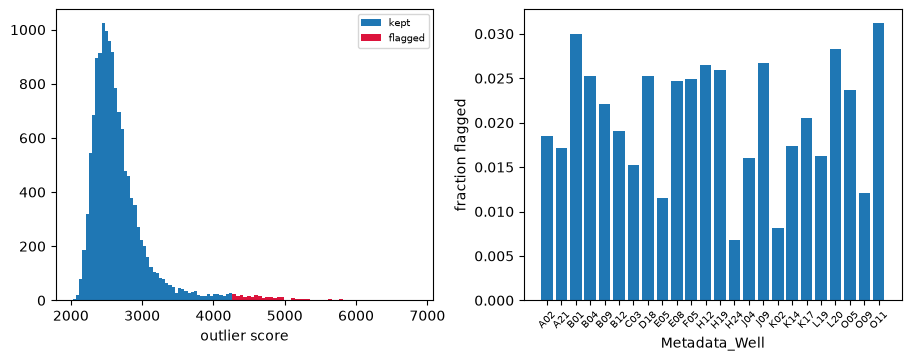
outliers() writes a flag and a score and removes nothing. The histogram shows the flagged tail of the score, and the bars the fraction flagged in each well. It scores only the features var["selected"] marks, so a block of near-duplicate features cannot outvote the rest.

The default method, ecod [Li et al., 2023], needs no tuning. A cell’s score is the sum over features of how far into a tail it sits, measured by rank, so the scale of a feature does not matter. isolation_forest catches cells that are unusual in their combination of features, and mad takes the largest robust z-score of any single feature, so score_cutoff=5 applies the usual five-robust-standard-deviations rule instead of a fixed fraction.

What gets flagged

Three measurements that are easy to picture, as percentiles within the plate:

features = ["Cells_AreaShape_Area", "Nuclei_AreaShape_Area", "Nuclei_Intensity_MeanIntensity_DNA"]
percentiles = mt.get.to_dataframe(jump, metadata=False, features=features).rank(pct=True)
percentiles.groupby(jump.obs["qc_outlier"]).median().round(2)

	Cells_AreaShape_Area	Nuclei_AreaShape_Area	Nuclei_Intensity_MeanIntensity_DNA
qc_outlier
False	0.51	0.51	0.49
True	0.06	0.07	0.97

Flagged cells are small, with small nuclei and bright DNA. Rounded cells look like that: cells in division, dying cells and fragments. Two fields of well O09 were imaged as well, and jump_plate() downloads them (44 MB), so the flagged cells there can be set beside cells that were kept. DNA is red, AGP green and Mito blue, and the white line is CellProfiler’s outline of the cell.

from spatialdata import get_pyramid_levels

plate = mt.ds.jump_plate()
imaged = jump.obs[(jump.obs["Metadata_Well"] == "O09") & jump.obs["Metadata_Site"].isin([1, 2])]
examples = {
    "flagged": imaged[imaged["qc_outlier"]].head(4),
    "kept": imaged[~imaged["qc_outlier"]].sample(4, random_state=0),
}

fig, axes = plt.subplots(2, 4, figsize=(10, 5))
for row, (label, cells_shown) in zip(axes, examples.items(), strict=True):
    row[0].set_title(label, loc="left")
    for ax, (_, cell) in zip(row, cells_shown.iterrows(), strict=False):
        field = f"BR00121438_O09_s{cell['Metadata_Site']}"
        mask = np.asarray(plate[f"{field}_cells"]) == cell["Metadata_ObjectNumber"]
        ys, xs = np.nonzero(mask)
        window = np.s_[max(ys.min() - 15, 0) : ys.max() + 15, max(xs.min() - 15, 0) : xs.max() + 15]
        image = get_pyramid_levels(plate[f"{field}_image"], n=0)
        rgb = np.stack([np.asarray(image.sel(c=c))[window] for c in ("DNA", "AGP", "Mito")], axis=-1).astype(float)
        ax.imshow((rgb / np.percentile(rgb, 99.5, axis=(0, 1))).clip(0, 1))
        ax.contour(mask[window], levels=[0.5], colors="white", linewidths=0.8)
for ax in axes.flat:
    ax.set_axis_off()
plt.show()

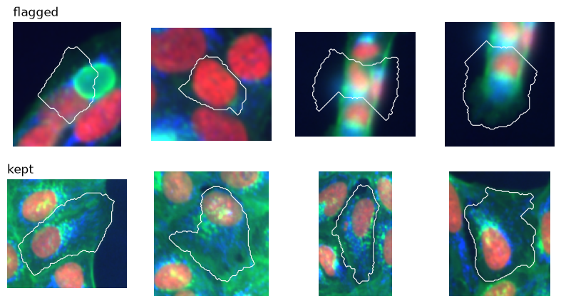
The kept cells are flat and spread out. The flagged ones are rounded, out of focus and badly outlined: the first outline covers the space beside a round cell rather than the cell, the second holds little but a nucleus, and the last two cut across a column of rounded cells. Their profiles describe the segmentation more than the cell.

The methods disagree

flags = {"ecod": jump.obs["qc_outlier"].to_numpy()}
for name, kwargs in {
    "ecod, paper": {"ecod_aggregation": "paper"},
    "isolation_forest": {"method": "isolation_forest"},
    "mad": {"method": "mad"},
}.items():
    mt.pp.outliers(jump, contamination=0.02, key_added="qc_compare", **kwargs)
    flags[name] = jump.obs["qc_compare"].to_numpy()

pd.DataFrame({a: {b: (flags[a] & flags[b]).sum() / (flags[a] | flags[b]).sum() for b in flags} for a in flags}).round(2)

	ecod	ecod, paper	isolation_forest	mad
ecod	1.00	0.79	0.81	0.21
ecod, paper	0.79	1.00	0.77	0.21
isolation_forest	0.81	0.77	1.00	0.24
mad	0.21	0.21	0.24	1.00

The table is the Jaccard index between flagged sets. ecod and isolation_forest flag largely the same cells. mad flags mostly others, because one extreme feature is enough for it. ecod_aggregation="paper" scores as Algorithm 1 of Li et al. [2023] does rather than as pyod does, and on these cells it shares most of its flags with the default.

Is it removing a phenotype?

per_well = jump.obs.groupby("Metadata_Well", observed=True).agg(
    control=("Metadata_Control", "first"), flagged=("qc_outlier", "mean")
)
per_well.groupby("control")["flagged"].agg(["count", "min", "median", "max"]).round(3)

	count	min	median	max
control
False	16	0.007	0.021	0.030
True	8	0.011	0.022	0.031

Control and compound wells lose similar fractions, between about 0.7 % and 3 % of a well, so here the flags do not concentrate on one compound’s wells. On a plate with a strong phenotype they may not: a compound that stops cells in division fills its wells with exactly the rounded cells flagged above. Look at this table before dropping anything. If one perturbation’s wells stand out, pass by="Metadata_Well" so each well is compared only with itself, or keep the cells.

Next: Normalize, select, aggregate.