Hits, effects and cell loss

This page asks which treatments moved away from the controls, which measurements changed, and whether a hit is a phenotype or cells that died. Hit calls come with a permutation p-value and feature effects with Mann-Whitney q-values.

Potency has its own page, Concentration response. The same questions asked of single cells are on What the well median hides.

import matplotlib.pyplot as plt
import scanpy as sc

import mantispy as mt

# Palette shared with the mantispy plotters (mt.pl.hits, mt.pl.cytotoxicity):
# crimson = significant / flagged, blue = ordinary / ok, grey = background.
ACCENT = "crimson"  # significant / flagged / highlighted (mt.pl.hits "hit")
ACCENT_DARK = "#7a1b1f"  # a second flagged compound, darker crimson
NEUTRAL = "tab:blue"  # ordinary / not-flagged (mt.pl.cytotoxicity "ok")
NULL = "lightgrey"  # not-significant / background (mt.pl.hits "not called")

import plotly.io as pio

pio.renderers.default = "notebook_connected"

A screen with replicates

pki is the JUMP pilot’s kinase inhibitor set: fifteen compounds in U2OS, eleven of them at three doses, with 32 to 64 replicate wells per treatment [Chandrasekaran et al., 2023]. That much replication is unusual, and it makes this a good place to see what a hit call does when the design is generous.

The preparation is the one from Normalize, select, aggregate.

wells = mt.ds.pki()
mt.pp.normalize(wells, by="Metadata_Plate", reference="negcon")
mt.pp.feature_select(wells, na_cutoff=0.0)
wells = mt.pp.subset_features(wells)
sc.pp.pca(wells, n_comps=20)
wells

AnnData object with n_obs × n_vars = 3072 × 850
    obs: 'Metadata_plate_map_name', 'Metadata_broad_sample', 'Metadata_mg_per_ml', 'Metadata_mmoles_per_liter', 'Metadata_solvent', 'Metadata_Plate', 'Metadata_Well', 'Metadata_Site_Count', 'Metadata_Count_Cells', 'Metadata_Count_CellsIncludingEdges', 'Metadata_Count_Cytoplasm', 'Metadata_Count_Nuclei', 'Metadata_Count_NucleiIncludingEdges', 'Metadata_Object_Count', 'Metadata_Barcode', 'Metadata_Supplier', 'Metadata_Supplier_Catalog', 'Metadata_pert_type', 'Metadata_control_type', 'Metadata_CellCount', 'Metadata_SiteCount', 'Metadata_Control', 'Metadata_Compound', 'Metadata_Concentration', 'Metadata_MOA', 'Metadata_Perturbation'
    var: 'object', 'feature_group', 'feature', 'channel', 'scale', 'angle', 'gray_levels', 'radial_bin', 'params', 'is_feature', 'degenerate_scale', 'selected'
    uns: 'mantispy', 'pca'
    obsm: 'X_pca'
    varm: 'PCs'
    layers: None (.X)

Calling hits

hit_calling() scores each group’s median distance from the control centroid, measured in the controls’ own covariance so that directions the controls already vary in count for less. The null is the other ways to draw a group of that size from the group and the held-out controls pooled.

With 850 features and 832 control wells, half of them held out, the covariance would be singular, so the distance is read on a PCA representation. The function says so itself if you forget.

mt.tl.hit_calling(wells, groupby="Metadata_Perturbation", use_rep="X_pca", n_permutations=1000)
mt.pl.hits(wells, label_top=6);

hits = wells.uns["mantispy"]["hits"].set_index("group")
hits.sort_values("distance", ascending=False).head(6)

	n_obs	distance	pvalue	qvalue	is_hit
group
BRD-U00086674-001-01-9@0.4	64	53.481017	0.000999	0.001265	True
BRD-U00086675-001-01-9@0.4	64	38.807105	0.000999	0.001265	True
BRD-K95785537-001-26-9@2.0	32	22.774036	0.000999	0.001265	True
BRD-U00086675-001-01-9@0.2	64	20.766895	0.000999	0.001265	True
BRD-U00086674-001-01-9@0.2	64	19.445404	0.000999	0.001265	True
BRD-K15179513-001-03-4@2.0	32	19.012001	0.000999	0.001265	True

# Every treatment's hit distance, reusing the table hit_calling already wrote (no recompute).
ranked = hits.sort_values("distance", ascending=False)
colours = [ACCENT if is_hit else NULL for is_hit in ranked["is_hit"]]

fig, ax = plt.subplots(figsize=(7, 4))
ax.bar(range(len(ranked)), ranked["distance"], color=colours, width=1.0)
ax.set_xticks([])
ax.set_xlabel("treatment, ranked by distance")
ax.set_ylabel("distance from controls")
ax.set_title("Hit distances across all treatments")
handles = [
    plt.Rectangle((0, 0), 1, 1, color=ACCENT),
    plt.Rectangle((0, 0), 1, 1, color=NULL),
]
ax.legend(handles, ["significant (is_hit)", "not significant"], frameon=False, fontsize=8)
fig.tight_layout()
plt.show()

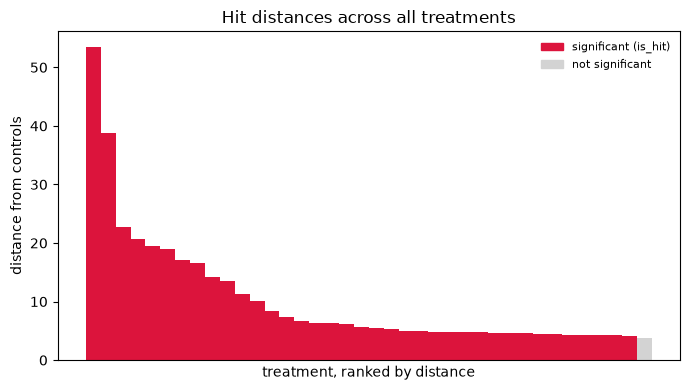
A handful of treatments tower over the rest, and the coloured bars are the ones whose permutation q-value clears significance; everything in grey below them is within reach of a control-sized draw.

Which features moved

A hit call says a treatment moved. It does not say what changed. effect_size() gives a per-feature effect against the controls with Mann-Whitney p-values, and one BH correction over the whole table.

mt.tl.effect_size(wells, groupby="Metadata_Perturbation", reference="negcon")
strongest = hits.drop(index="DMSO")["distance"].idxmax()

mt.pl.feature_volcano(wells, group=strongest);

import numpy as np

# Reuse the effect-size table tl.effect_size already wrote; do not recompute.
effects = wells.uns["mantispy"]["effect"]
top_hits = hits.drop(index="DMSO").sort_values("distance", ascending=False).head(8).index.tolist()

grid = effects[effects["group"].isin(top_hits)].pivot(index="feature", columns="group", values="effect")[top_hits]
top_features = grid.abs().max(axis=1).sort_values(ascending=False).head(18).index
grid = grid.loc[top_features]

_COMPARTMENTS = ("Cytoplasm_", "Nuclei_", "Cells_")
_CHANNELS = ("DNA", "ER", "RNA", "AGP", "Mito", "Brightfield")


def short(name):
    """Shorten a CellProfiler feature name to its family and channel, dropping the compartment prefix and trailing indices."""
    label = name
    for prefix in _COMPARTMENTS:
        if label.startswith(prefix):
            label = label[len(prefix) :]
            break
    parts = label.split("_")
    channels = [p for p in parts if p in _CHANNELS]
    if channels:
        family = parts[: parts.index(channels[0])]
        return "_".join(family) + " " + " ".join(channels)
    while parts and parts[-1].isdigit():
        parts.pop()
    return "_".join(parts)


def tick(group):
    """Shorten a treatment label to its first two compound tokens plus the dose."""
    head, dose = group.split("@")
    return "-".join(head.split("-")[:2]) + "@" + dose


vmax = float(np.nanmax(np.abs(grid.to_numpy())))
fig, ax = plt.subplots(figsize=(7, 5.5))
im = ax.imshow(grid.to_numpy(), aspect="auto", cmap="RdBu_r", vmin=-vmax, vmax=vmax)
ax.set_xticks(range(grid.shape[1]))
ax.set_xticklabels([tick(g) for g in grid.columns], rotation=90, fontsize=7)
ax.set_yticks(range(grid.shape[0]))
ax.set_yticklabels([short(f) for f in grid.index], fontsize=7)
fig.colorbar(im, ax=ax, label="signed effect size (Cohen's d)")
ax.set_title("Shared feature responses across the top hits")
fig.tight_layout()
plt.show()

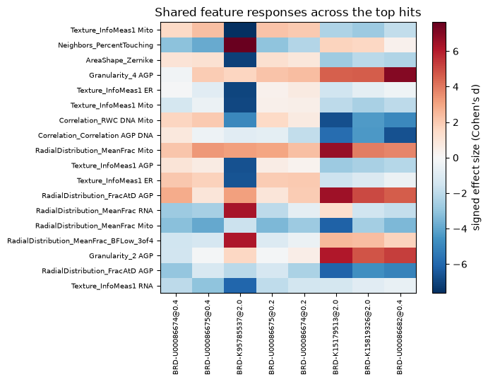
Columns that share a red-and-blue pattern move the same features in the same direction, which is the raw material for asking whether two compounds share a mechanism in Mechanism of action.

Each point is one CellProfiler measurement. The named ones are where this compound’s effect lives, and they are the handle for the next question, whether two compounds move the same features, which is Mechanism of action.

One profile per perturbation

Replicate wells of a treatment are combined into a signature with consensus().

signatures = mt.tl.consensus(wells, by="Metadata_Perturbation", method="median")
print(f"{wells.n_obs} wells -> {signatures.n_obs} signatures")
signatures

3072 wells -> 38 signatures

AnnData object with n_obs × n_vars = 38 × 850
    obs: 'Metadata_Perturbation', 'Metadata_ReplicateCount', 'Metadata_plate_map_name', 'Metadata_broad_sample', 'Metadata_mg_per_ml', 'Metadata_mmoles_per_liter', 'Metadata_solvent', 'Metadata_Site_Count', 'Metadata_Barcode', 'Metadata_Supplier', 'Metadata_Supplier_Catalog', 'Metadata_pert_type', 'Metadata_control_type', 'Metadata_Control', 'Metadata_Compound', 'Metadata_Concentration', 'Metadata_MOA'
    var: 'object', 'feature_group', 'feature', 'channel', 'scale', 'angle', 'gray_levels', 'radial_bin', 'params', 'is_feature', 'degenerate_scale', 'selected'
    uns: 'mantispy'
    layers: None (.X)

import numpy as np

# Median pairwise Pearson correlation among each treatment's replicate wells (treated wells only).
treated = wells[~wells.obs["Metadata_Control"].to_numpy(dtype=bool)]
matrix = np.asarray(treated.X, dtype=float)
agreement = []
for members in treated.obs.groupby("Metadata_Perturbation", observed=True).indices.values():
    if len(members) < 3:
        continue
    corr = np.corrcoef(matrix[members])
    upper = np.triu_indices(len(members), 1)
    agreement.append(np.nanmedian(corr[upper]))

fig, ax = plt.subplots(figsize=(6, 4))
ax.hist(agreement, bins=20, color=ACCENT)
ax.set_xlabel("median replicate correlation")
ax.set_ylabel("treatments")
ax.set_title("How consistent are replicate wells")
fig.tight_layout()
plt.show()

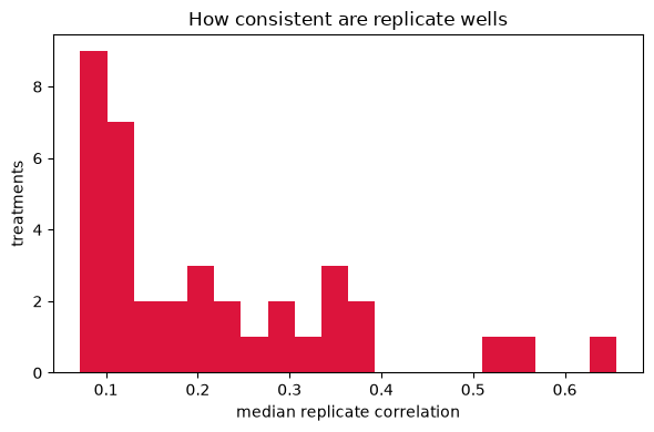
Most treatments’ replicates agree closely, so a plain median loses little; the low-correlation tail is where replicates disagree and where modz, by down-weighting off-consensus wells, earns its keep.

median is the default and is what pycytominer does by default. modz weights each replicate by how well it agrees with the others, which helps when replicates are few and noisy.

Is it a hit, or did the cells die?

A compound that kills four fifths of the cells leaves a well median computed from a fifth as many cells, and that median moves away from the controls for reasons unrelated to the biology being screened. It looks like a strong hit.

The cell count is also a baseline to beat. Seal et al. [2025] found that across three bioactivity benchmarks a model given only the cell count often matched one given the whole Cell Painting profile, and Ewald et al. [2026] found that profiles predicted LDH release no better than cell count, plate and well position.

cytotoxicity() reads the two together: each group’s viability, its cells per field against the controls’, beside its median distance from the controls.

mt.tl.cytotoxicity(wells)
wells.uns["mantispy"]["cytotoxicity"].round(3)

	group	n_obs	viability	distance	suspect
0	BRD-K15179513-001-03-4@2.0	32	0.783	19.012	False
1	BRD-K15819326-001-01-6@2.0	32	0.840	17.161	False
2	BRD-K40109029-001-06-9@2.0	32	0.831	14.228	False
3	BRD-K95785537-001-26-9@2.0	32	0.763	22.774	False
4	BRD-U00086672-001-01-9@0.2	64	1.030	4.241	False
5	BRD-U00086672-001-01-9@0.4	64	1.012	4.442	False
6	BRD-U00086672-001-01-9@1.0	64	0.983	5.735	False
7	BRD-U00086673-001-01-9@0.2	64	0.998	4.772	False
8	BRD-U00086673-001-01-9@0.4	64	0.988	5.009	False
9	BRD-U00086673-001-01-9@1.0	64	0.972	5.461	False
10	BRD-U00086674-001-01-9@0.04	64	0.973	6.201	False
11	BRD-U00086674-001-01-9@0.2	64	0.676	19.445	True
12	BRD-U00086674-001-01-9@0.4	64	0.266	53.481	True
13	BRD-U00086675-001-01-9@0.04	64	0.935	6.763	False
14	BRD-U00086675-001-01-9@0.2	64	0.497	20.767	True
15	BRD-U00086675-001-01-9@0.4	64	0.331	38.807	True
16	BRD-U00086676-001-01-9@0.004	64	0.968	10.128	False
17	BRD-U00086676-001-01-9@0.01	64	0.973	11.316	False
18	BRD-U00086676-001-01-9@0.04	64	0.931	13.587	False
19	BRD-U00086677-001-01-9@0.004	64	1.013	4.255	False
20	BRD-U00086677-001-01-9@0.01	64	1.008	4.218	False
21	BRD-U00086677-001-01-9@0.04	64	0.997	4.570	False
22	BRD-U00086678-001-01-9@0.004	64	0.979	4.861	False
23	BRD-U00086678-001-01-9@0.01	64	0.996	4.604	False
24	BRD-U00086678-001-01-9@0.04	64	1.005	5.245	False
25	BRD-U00086679-001-01-9@0.2	64	0.990	4.406	False
26	BRD-U00086679-001-01-9@0.4	64	0.991	4.747	False
27	BRD-U00086679-001-01-9@1.0	64	1.044	5.043	False
28	BRD-U00086680-001-01-9@0.04	64	1.000	4.337	False
29	BRD-U00086680-001-01-9@0.2	64	1.000	6.274	False
30	BRD-U00086680-001-01-9@0.4	64	1.005	7.280	False
31	BRD-U00086681-001-01-9@0.04	64	1.005	4.183	False
32	BRD-U00086681-001-01-9@0.2	64	0.994	4.689	False
33	BRD-U00086681-001-01-9@0.4	64	1.049	4.843	False
34	BRD-U00086682-001-01-9@0.04	64	1.030	6.348	False
35	BRD-U00086682-001-01-9@0.2	64	0.983	8.459	False
36	BRD-U00086682-001-01-9@0.4	64	0.941	16.629	False
37	DMSO	832	1.000	3.880	False

mt.pl.cytotoxicity(wells);

# Join the cytotoxicity table to each treatment's compound and dose, then follow the flagged compounds down the ladder.
cyto = wells.uns["mantispy"]["cytotoxicity"]
meta = wells.obs.groupby("Metadata_Perturbation", observed=True)[
    ["Metadata_Compound", "Metadata_Concentration"]
].first()
viability_table = cyto.join(meta, on="group")
flagged = viability_table.loc[viability_table["suspect"], "Metadata_Compound"].unique()

# These are the same two compounds mt.pl.cytotoxicity draws as crimson "suspect" points above.
# Colour them in crimson too, the more-toxic one (lowest surviving fraction) in ACCENT and the
# second in a darker crimson, so the reader connects the two figures.
toxicity = viability_table[viability_table["Metadata_Compound"].isin(flagged)]
order = toxicity.groupby("Metadata_Compound", observed=True)["viability"].min().sort_values().index
palette = dict(zip(order, [ACCENT, ACCENT_DARK], strict=False))

fig, ax = plt.subplots(figsize=(6, 4))
for compound in flagged:
    block = viability_table[viability_table["Metadata_Compound"] == compound].sort_values(
        "Metadata_Concentration", key=lambda s: s.astype(float)
    )
    dose = block["Metadata_Concentration"].astype(float)
    label = "-".join(str(compound).split("-")[:2])
    ax.plot(dose, block["viability"], marker="o", color=palette[compound], label=label)
ax.axhline(1.0, color="0.7", lw=1, ls="--")
ax.set_xscale("log")
ax.set_xlabel("dose (Metadata_Concentration)")
ax.set_ylabel("viability (cells per field vs controls)")
ax.set_title("Viability falls at the top doses")
ax.legend(frameon=False, fontsize=8)
fig.tight_layout()
plt.show()

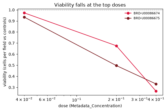
Both flagged compounds keep a control-sized complement of cells at their lowest dose and lose most of it at the top two, which is the confound tl.cytotoxicity marks: a large distance at high dose is partly cells dying rather than phenotype.

Two compounds are flagged, each at its two highest doses, which keep between 27% and 68% of the controls’ cells. The strongest, BRD-U00086674 at 0.4, keeps 27% of its cells and sits further from the controls than any other treatment. At its lowest dose, 0.04, its cells survive and it sits close to the controls.

Both conditions have to hold. Cell loss alone is a phenotype (a compound that arrests growth is a real finding), and a large distance alone is a hit. Only the combination is suspect. tl.cytotoxicity is a diagnostic and does not correct anything.

Summary

• A hit call says a treatment moved away from the controls. effect_size() says which features moved, and consensus() gives one signature per treatment.

• Cell loss and phenotype are confounded by construction. Flag the combination with cytotoxicity() instead of correcting it away.

Next: Mechanism of action, which asks whether two treatments moved the same way.