Which measurements moved

A hit call says a perturbation moved, and a mechanism call says what it resembles. Neither says what changed in the cell. This page tests features against the controls, collapses them into families a biologist can read, and lends names to the axes of an embedding, which has none of its own.

import matplotlib.pyplot as plt
import numpy as np
import pandas as pd
from scipy import stats

import scanpy as sc

import mantispy as mt

import plotly.io as pio

pio.renderers.default = "notebook_connected"

Test the unit that was randomized

A well of a few hundred cells is not a few hundred independent observations of a treatment. The cells share the well’s confluency, focus and plate position. Single-cell transcriptomics settled on pseudobulk for this: aggregate to the unit that was randomized, then test.

The cost of ignoring this can be measured on wells where nothing differs. Take the eight DMSO wells of the JUMP plate in jump_cells(), split them into two halves of four, and test the halves against each other, once cell by cell and once on the well medians. Every feature called is a false positive by construction.

from mantispy._core._stats import benjamini_hochberg

cells = mt.ds.jump_cells(selected=True)
mt.pp.normalize(cells, method="mad_robustize", by="Metadata_Plate", reference="negcon")
controls = cells[cells.obs["Metadata_Control"].to_numpy()].copy()

values = np.asarray(controls.X, dtype=float)
values = values[:, np.isfinite(values).all(axis=0)]
well = controls.obs["Metadata_Well"].astype(str).to_numpy()
names = sorted(set(well))
left = np.isin(well, names[::2])

_, per_cell = stats.mannwhitneyu(values[left], values[~left], axis=0)
medians = pd.DataFrame(values).groupby(well).median()
on_left = medians.index.isin(names[::2])
_, per_well = stats.ttest_ind(medians[on_left], medians[~on_left], axis=0)

{
    "control wells": len(names),
    "cells": len(well),
    "features": values.shape[1],
    "called at q < 0.05, cell by cell": int((benjamini_hochberg(per_cell) < 0.05).sum()),
    "called at q < 0.05, on well medians": int((benjamini_hochberg(per_well) < 0.05).sum()),
}

{'control wells': 8,
 'cells': 5421,
 'features': 1598,
 'called at q < 0.05, cell by cell': 677,
 'called at q < 0.05, on well medians': 0}

counts = {
    "cell by cell": int((benjamini_hochberg(per_cell) < 0.05).sum()),
    "on well medians": int((benjamini_hochberg(per_well) < 0.05).sum()),
}
fig, ax = plt.subplots(figsize=(5, 4))
bars = ax.bar(list(counts), list(counts.values()), color=["indianred", "steelblue"])
ax.bar_label(bars, padding=2)
ax.set_ylabel("features called at q < 0.05")
ax.set_title(f"Two halves of the control wells ({values.shape[1]} features)")
fig.tight_layout()
plt.show()

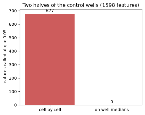
Bars are the number of features called different between two halves of the DMSO wells, where nothing differs. The per-cell test calls hundreds; the test on well medians calls none.

Cell by cell, 677 of 1,598 features differ between two halves of the DMSO wells, where nothing differs. On the well medians, none do. The cells of a well share its confluency, focus and position, so a per-cell test counts a few hundred correlated observations as independent evidence.

For this reason tl.differential_features rejects cell-resolution input and points to tl.aggregate. The same applies to tl.rank_features, which does run per cell: it is the right tool only when the cells themselves are the population you are describing, not when they are replicates of a treatment.

try:
    mt.tl.differential_features(cells)
except ValueError as error:
    print(error)

differential_features needs well-level profiles; testing per cell treats cells as independent replicates and inflates the false discovery rate. Aggregate first with adata = mt.tl.aggregate(adata).

The p-value floor of a rank test

effect_size() computes a Mann-Whitney p-value per feature and group. A rank test’s resolution is limited by the number of observations: with few treated wells there are only so many ways to interleave them with the controls, so there is a smallest p-value it can produce, however large the effect. The treated values below all lie above every control, the largest effect the test can see.

control = np.arange(300, dtype=float)
wells = [2, 3, 4, 6, 8]
smallest_p = [stats.mannwhitneyu(np.arange(n, dtype=float) + 1e6, control).pvalue for n in wells]
fig, ax = plt.subplots(figsize=(5, 4))
ax.plot(wells, smallest_p, marker="o", color="steelblue")
ax.axhline(5e-7, color="grey", ls="--", lw=1, label="~5e-7 correction threshold")
ax.set_yscale("log")
ax.set_xlabel("treated wells")
ax.set_ylabel("smallest possible p-value")
ax.set_title("Rank-test p-value floor")
ax.legend(fontsize=8)
fig.tight_layout()
plt.show()

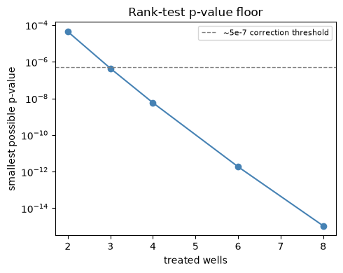
Smallest p-value a Mann-Whitney can return, against the number of treated wells (log y). It falls as wells increase; at two wells it is above the dashed reference line, at four it is below.

control = np.arange(300, dtype=float)
floor = pd.DataFrame(
    [
        {
            "treated wells": n,
            # Distinct values, not np.full: identical treated wells tie with each other,
            # and scipy answers a tied sample with the normal approximation instead of the
            # exact null, which gives a different, much larger number.
            "smallest possible p": stats.mannwhitneyu(np.arange(n, dtype=float) + 1e6, control).pvalue,
        }
        for n in (2, 3, 4, 6, 8)
    ]
)
floor["smallest possible p"] = floor["smallest possible p"].map("{:.2e}".format)
floor

	treated wells	smallest possible p
0	2	4.40e-05
1	3	4.36e-07
2	4	5.73e-09
3	6	1.84e-12
4	8	1.09e-15

A screen testing a few hundred genes across a few hundred features runs on the order of 10⁵ tests, so the top-ranked test needs a p-value of about 5e-07 to survive multiple-testing correction. At two wells the floor is a hundred times too large, so no effect of any size can be called. At three it is the same order as the threshold, and at four it no longer limits anything.

differential_features() fits a moderated t-test instead, with wells as the replicates, and has no such floor. diagnose_testing() checks both on your own screen: the rank test’s resolution against the number of tests, and whether the parametric p-values are calibrated, by relabelling control wells as pseudo-treatments.

On a real screen

rohban is an ORF overexpression screen: one gene per well, about ten replicate wells per gene over five plates. Its untransfected wells are neither a gene nor a control, so they go first.

adata = mt.ds.rohban()
adata = adata[adata.obs["Metadata_gene_name"] != "EMPTY"].copy()
mt.pp.normalize(adata, method="mad_robustize", by="Metadata_Plate", reference="negcon")
mt.pp.feature_select(adata, na_cutoff=0.0)
adata = mt.pp.subset_features(adata)

mt.metrics.diagnose_testing(adata)

	check	value	expected	verdict	note
0	wells per treatment	10 (min 4)	>= 3	pass	the unit that was randomized, and the sample s...
1	treatments sharing a Metadata_Plate with the r...	190 of 190	all	pass	median 5 Metadata_Plate per treatment
2	excess kurtosis	44.0	0 (Gaussian)	warn	heavy tails break the small p-values first; mt...
3	rank test resolution	1.6e-07	< 3.4e-07	pass	smallest p a Mann-Whitney can return with 10 w...
4	null p < 0.05	7.4%	5%	pass	control wells relabeled as 10-well treatments,...
5	null p < 0.01	3.1%	1%	FAIL	control wells relabeled as 10-well treatments,...
6	null discoveries	1 of 6,128	0	FAIL	findings on data where there is nothing to find
7	hit_calling null rate	1 of 8	<= 2	pass	hit_calling called a control-only pseudo-treat...
8	edistance null rate	2 of 8	<= 2	pass	edistance called a control-only pseudo-treatme...

At ten wells per gene the rank test has all the resolution it needs. The parametric test’s tail does not hold: control wells relabelled as ten-well treatments fall below p = 0.01 three times as often as they should, and a false discovery survives the correction on data where there is nothing to find. The features are heavy-tailed, with an excess kurtosis of 44 where a Gaussian has none. Rank-transform them and check again:

mt.pp.rank_int(adata)
mt.metrics.diagnose_testing(adata)

	check	value	expected	verdict	note
0	wells per treatment	10 (min 4)	>= 3	pass	the unit that was randomized, and the sample s...
1	treatments sharing a Metadata_Plate with the r...	190 of 190	all	pass	median 5 Metadata_Plate per treatment
2	excess kurtosis	-0.0	0 (Gaussian)	pass	heavy tails break the small p-values first; mt...
3	rank test resolution	1.6e-07	< 3.4e-07	pass	smallest p a Mann-Whitney can return with 10 w...
4	null p < 0.05	5.5%	5%	pass	control wells relabeled as 10-well treatments,...
5	null p < 0.01	0.9%	1%	pass	control wells relabeled as 10-well treatments,...
6	null discoveries	0 of 6,128	0	pass	findings on data where there is nothing to find
7	hit_calling null rate	0 of 8	<= 2	pass	hit_calling called a control-only pseudo-treat...
8	edistance null rate	0 of 8	<= 2	pass	edistance called a control-only pseudo-treatme...

After rank_int() every check passes: 0.9% of the null falls below p = 0.01 and nothing is discovered on it. The transform is also a step of the consortium’s compound recipe.

mt.tl.differential_features(adata, groupby="Metadata_Gene", block="Metadata_Plate")
table = adata.uns["mantispy"]["differential"]
called = table[table["qvalue"] < 0.05]
print(
    f"{len(called)} of {len(table)} tests called at q < 0.05, in {called['group'].nunique()} of {table['group'].nunique()} genes"
)
called.sort_values("qvalue").head(8)

33793 of 145540 tests called at q < 0.05, in 189 of 190 genes

	group	feature	difference	t	pvalue	qvalue
109128	RAF1	Cytoplasm_Intensity_LowerQuartileIntensity_RNA	2.766217	12.549329	1.337704e-26	1.946894e-21
108973	RAF1	Cells_RadialDistribution_RadialCV_RNA_3of4	-2.380923	-12.394384	3.866567e-26	2.813701e-21
27808	CEBPA	Cells_Texture_InfoMeas1_ER_5_02_256	3.175778	11.954069	9.625190e-25	4.669500e-20
27604	CEBPA	Cells_Correlation_Correlation_AGP_DNA	-3.079383	-11.892230	1.463139e-24	5.323631e-20
18740	BRAF	Cytoplasm_Intensity_LowerQuartileIntensity_RNA	2.622494	11.707125	4.452446e-24	8.100112e-20
49370	ERG	Cytoplasm_Granularity_8_DNA	3.107021	11.784207	3.488408e-24	8.100112e-20
66833	JUN	Cells_RadialDistribution_RadialCV_DNA_4of4	2.875414	11.777718	3.451884e-24	8.100112e-20
108806	RAF1	Cells_Correlation_Correlation_DNA_RNA	-2.544252	-11.703200	4.330589e-24	8.100112e-20

# feature_volcano reads an effect table (group, feature, effect, qvalue). The moderated-t contrast above is
# that effect, so expose the differential table under the key the plot looks for rather than rerun a rank test.
adata.uns["mantispy"]["effect"] = adata.uns["mantispy"]["differential"].rename(columns={"difference": "effect"})

mt.pl.feature_volcano(adata, group="RAF1");

Each point is one feature tested for RAF1, a gene at the top of the table: x is the effect size versus DMSO, y is -log10 of the q-value, and colour is the feature family. The points spread to both signs, and the counts beside the q < 0.05 line say how many features cleared it.

Nearly every gene moves some features: with ten wells per gene the test has the power to call small, consistent shifts. The top of the table already reads as biology. RAF1 and BRAF, two kinases of the same MAPK cascade, both raise the same feature, the lower quartile of cytoplasmic RNA intensity. A table of tens of thousands of calls says that a lot changed, not what; the next sections read it by family.

What blocking on plate does

differential_features takes block=, which adds the plate to the model as a fixed effect. On data that was not normalized per plate it recovers the power plate variance would cost. It also refuses a confounded layout: if a perturbation’s wells sit only on plates without control wells, its treatment and its plate are the same variable and no test can separate them.

BBBC021 shows what that looks like, and the rest of this page uses the screen, because its mechanisms give the signatures below something to be read against. Lactacystin at 10 uM sits on three plates, which hold 18 DMSO wells between them.

bbbc = mt.ds.bbbc021()
mt.pp.normalize(bbbc, method="mad_robustize", by="Metadata_Plate", reference="negcon")
mt.pp.feature_select(bbbc, na_cutoff=0.0)
bbbc = mt.pp.subset_features(bbbc)

lactacystin = (bbbc.obs["Metadata_Perturbation"] == "lactacystin@10.0").to_numpy()
plates = set(bbbc.obs.loc[lactacystin, "Metadata_Plate"])
{
    "lactacystin@10.0 wells": int(lactacystin.sum()),
    "on plates": sorted(plates),
    "DMSO wells on those plates": int((bbbc.obs["Metadata_Control"] & bbbc.obs["Metadata_Plate"].isin(plates)).sum()),
}

{'lactacystin@10.0 wells': 3,
 'on plates': ['Week6_31641', 'Week6_31661', 'Week6_31681'],
 'DMSO wells on those plates': 18}

# Had QC dropped the DMSO wells of those three plates, lactacystin's plates would hold no controls.
lost = bbbc.obs["Metadata_Control"].to_numpy() & bbbc.obs["Metadata_Plate"].isin(plates).to_numpy()
confounded = bbbc[(lactacystin | bbbc.obs["Metadata_Control"].to_numpy()) & ~lost].copy()
mt.tl.differential_features(confounded, block=None, key_added="unblocked")
unblocked = confounded.uns["mantispy"]["unblocked"]
print(f"unblocked: {(unblocked['qvalue'] < 0.05).sum()} of {len(unblocked)} features called")

try:
    mt.tl.differential_features(confounded, block="Metadata_Plate")
except ValueError as error:
    print(f"blocked:   {error}")

unblocked: 77 of 343 features called
blocked:   no group had enough replicates in blocks shared with the reference

With the DMSO wells of lactacystin’s three plates removed, the unblocked test calls 77 of 343 features, and any of them could be the plate. Blocked on plate, the test refuses, because no lactacystin well then shares a plate with a control.

From features to feature families

A differential table has one row per (perturbation, feature), and a screen has thousands of features, so the table does not directly say what a compound did. Biologists read results at the level of feature families, such as intensity in the tubulin channel or texture in the nucleus. tl.feature_signature collapses the table into families and keeps the sign.

mt.tl.differential_features(bbbc, key_added="vs_dmso")
signature = mt.tl.feature_signature(bbbc, key="vs_dmso")
signature

AnnData object with n_obs × n_vars = 103 × 19
    obs: 'Metadata_Perturbation', 'Metadata_Plate', 'Metadata_Well', 'Metadata_Compound', 'Metadata_Concentration', 'Metadata_MOA', 'Metadata_CellCount', 'Metadata_SiteCount', 'Metadata_Control'
    var: 'object', 'feature_group', 'feature', 'channel', 'scale', 'angle', 'gray_levels', 'radial_bin', 'params', 'is_feature', 'n_features'
    uns: 'mantispy'
    layers: None (.X)

mt.pl.feature_signature(signature, groupby="Metadata_MOA");

# sets_heatmap reads per-well enrichment scores, so score the same feature families the signature collapses to.
mt.tl.enrich(bbbc, by=["feature_group", "channel", "object"])

mt.pl.sets_heatmap(bbbc, groupby="Metadata_MOA");

Mean enrichment score per mechanism across the feature families the signature collapses to (rows = mechanisms, columns = families, colour = mean score on a diverging scale). Each mechanism lights up its own set of families, and the cytoskeleton channels stand out.

families = mt.get.to_dataframe(signature, metadata=False).astype(float)
by_mechanism = families.groupby(signature.obs["Metadata_MOA"].astype(str).to_numpy()).mean()
mechanisms = ("Microtubule stabilizers", "Microtubule destabilizers", "Eg5 inhibitors", "Actin disruptors")
{mechanism: by_mechanism.loc[mechanism].nlargest(2).round(1).to_dict() for mechanism in mechanisms}

{'Microtubule stabilizers': {'Intensity | CorrActin | Nuclei': 11.4,
  'Intensity | CorrTub | Cytoplasm': 11.1},
 'Microtubule destabilizers': {'Intensity | CorrActin | Nuclei': 11.6,
  'Intensity | CorrActin | Cytoplasm': 7.0},
 'Eg5 inhibitors': {'Intensity | CorrActin | Nuclei': 12.5,
  'Intensity | CorrTub | Nuclei': 9.3},
 'Actin disruptors': {'Intensity | CorrTub | Cytoplasm': 11.6,
  'Intensity | CorrTub | Cells': 10.6}}

Compare the rows with what each stain shows. The mechanisms move the cytoskeleton channels, and not always the one their target sits in. Actin intensity over the nucleus is the largest change for microtubule destabilizers and Eg5 inhibitors, and about level with tubulin intensity in the cytoplasm for microtubule stabilizers, while the actin disruptors change tubulin intensity most. The two cytoskeletons are mechanically coupled, and a cell arrested in mitosis rounds up over its nucleus.

So look at the signature instead of assuming it. A drug that targets X does not necessarily cause its largest measured change in channel X.

The other contrast, contrast="rest", tests each treatment against every other one rather than against the controls. That subtracts what a treatment shares with all the others, including the ones with the same mechanism, so it makes a single treatment distinctive and blurs its mechanism group. Use contrast="rest" to tell perturbations apart and contrast="reference", as in the figure, to find which ones belong together.

enrich() scores the same families on consensus profiles with decoupler, as the overview does.

When the features have no names

The hardest thing about an embedding is that a result has no vocabulary. A CellProfiler hit comes with “nuclear texture went down”; an embedding hit comes with a compound ID and nothing else.

JUMP-Lite lets you fix that cleanly, because the same wells were measured both ways. Use the named block to name the unnamed one: regress every CellProfiler measurement on the embedding’s components and ask how much of it the embedding already carries.

One thing to get right first. ds.jump_lite returns the six blocks in one row order, but the files it reads list the wells in six different orders, and so will most tables from different pipelines. Stacking two blocks positionally is then silent and wrong, so align on the index.

def embedded(model):
    """One JUMP-Lite embedding, normalized per plate and reduced to its first 50 components."""
    wells = mt.ds.jump_lite(model)
    mt.pp.normalize(wells, method="mad_robustize", by="Metadata_Plate", reference="negcon")
    mt.pp.feature_select(wells, operations=("drop_degenerate", "drop_na_columns"), na_cutoff=0.0)
    wells = mt.pp.subset_features(wells)
    sc.pp.pca(wells, n_comps=50)
    return wells


blocks = {model: embedded(model) for model in ("openphenom", "dinov2", "dinov2_random")}

embedding = blocks["openphenom"]

# The question is how much of each named measurement the embedding carries, so keep them all and drop only
# the runaway ones.
named = mt.ds.jump_lite("cp_measure")
mt.pp.normalize(named, method="mad_robustize", by="Metadata_Plate", reference="negcon")
mt.pp.feature_select(named, operations=("drop_degenerate", "drop_na_columns", "drop_outliers"), na_cutoff=0.0)
named = mt.pp.subset_features(named)

aligned = named[named.obs_names.get_indexer(embedding.obs_names)].copy()
{
    "named measurements kept": named.n_vars,
    "same set of wells": set(embedding.obs_names) == set(named.obs_names),
    "rows out of OpenPhenom's order, per block": {
        model: int((wells.obs_names != embedding.obs_names).sum()) for model, wells in blocks.items()
    },
}

{'named measurements kept': 1857,
 'same set of wells': True,
 "rows out of OpenPhenom's order, per block": {'openphenom': 0,
  'dinov2': 0,
  'dinov2_random': 0}}

from sklearn.linear_model import RidgeCV
from sklearn.model_selection import KFold


def standard(block):
    """Centre and scale each column, leaving a column that never varies alone rather than dividing by zero."""
    spread = block.std(0)
    return (block - block.mean(0)) / np.where(spread > 0, spread, 1)


measurements = standard(np.asarray(aligned.X, dtype=float))


def carried(wells):
    """Out-of-fold R^2 of every CellProfiler measurement, predicted from this block's components."""
    # Put each block into the order `aligned` is in rather than trusting the two to match. When they do not,
    # skipping this is silent: the regression simply finds nothing, and an informative block scores like a random one.
    X = np.asarray(wells[wells.obs_names.get_indexer(aligned.obs_names)].obsm["X_pca"], dtype=float)
    Y = measurements

    predicted = np.zeros_like(Y)
    for train, test in KFold(5, shuffle=True, random_state=0).split(X):
        predicted[test] = RidgeCV(alphas=np.logspace(-1, 4, 12)).fit(X[train], Y[train]).predict(X[test])
    return pd.Series(1 - ((Y - predicted) ** 2).sum(0) / (Y**2).sum(0), index=aligned.var_names)


explained = pd.DataFrame({name: carried(blocks[name]) for name in ("openphenom", "dinov2", "dinov2_random")})
explained["feature_group"] = aligned.var["feature_group"].to_numpy()
explained["object"] = aligned.var["object"].to_numpy()

by_group = explained.groupby("feature_group", observed=True)[["openphenom", "dinov2", "dinov2_random"]].median()
by_group.sort_values("openphenom", ascending=False).round(3)

	openphenom	dinov2	dinov2_random
feature_group
texture	0.816	0.747	0.235
ferret	0.637	0.683	0.160
intensity	0.617	0.594	0.152
radial_distribution	0.551	0.542	0.179
radial_zernikes	0.491	0.522	0.152
sizeshape	0.484	0.592	0.010
zernike	0.472	0.516	0.152

fig, ax = plt.subplots(figsize=(8, 4))
panel = by_group.sort_values("openphenom")
positions = np.arange(len(panel))
for offset, name, colour in (
    (-0.26, "openphenom", "steelblue"),
    (0.0, "dinov2", "seagreen"),
    (0.26, "dinov2_random", "lightgrey"),
):
    ax.barh(positions + offset, panel[name], 0.25, label=name, color=colour)
ax.set_yticks(positions, panel.index, fontsize=9)
ax.set_xlabel("out-of-fold $R^2$ of the CellProfiler measurement, from the embedding")
ax.legend(fontsize=8)
fig.tight_layout()
plt.show()

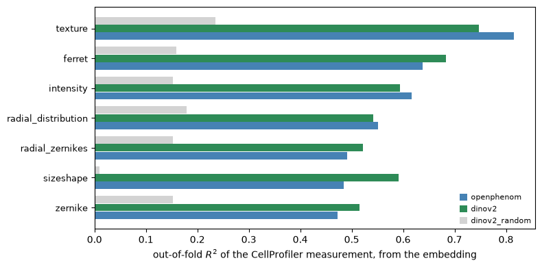
That is a vocabulary for the embedding, and it is specific enough to act on. Both trained models reconstruct the texture measurements best, and the untrained model reconstructs little of anything — the gap between the grey bars and the coloured ones is what training bought, measured in units a CellProfiler user already understands.

Read that as a hint about which biology an embedding is built to see. Texture is the part of the named profile both trained models carry best, so a phenotype that shows up mainly as a change of staining texture is the kind most likely to survive swapping in an embedding. Which phenotypes that covers in a given assay is a question for the assay, not for this table.

The two models agree on more than texture: both carry the Feret diameters second-best. They part most on the size-and-shape measurements, which DINOv2 carries noticeably better than OpenPhenom does. So “an embedding” is not one thing, and swapping one for another changes which phenotypes you can see; check your phenotype’s family against the model you plan to use. Only these two trained models were regressed here, so this says nothing yet about SubCell or MorphEm.

The floor is not zero, either. An untrained network still carries some of a named measurement, which is why the untrained control belongs in this plot as much as in the JUMP-Lite benchmark.

The same trick names the leading components, as far as it goes.

components = np.asarray(embedding.obsm["X_pca"])[:, :5]
values = np.asarray(aligned.X, dtype=float)
usable = np.isfinite(values).all(0) & (values.std(0) > 0)

# standard() is the one defined above, so the two tables are scaled the same way.
correlation = standard(components).T @ standard(values[:, usable]) / len(components)
names = aligned.var_names[usable]

rows = []
for index in range(components.shape[1]):
    best = np.argmax(np.abs(correlation[index]))
    rows.append(
        {
            "component": f"PC{index + 1}",
            "variance": round(float(embedding.uns["pca"]["variance_ratio"][index]), 3),
            "r with cell count": round(
                float(np.corrcoef(components[:, index], embedding.obs["Metadata_CellCount"])[0, 1]), 2
            ),
            "best named match": names[best],
            "r": round(float(correlation[index, best]), 2),
        }
    )
pd.DataFrame(rows).set_index("component")

	variance	r with cell count	best named match	r
component
PC1	0.635	-0.70	nuclei_3/max/radial_zernikesRadialDistribution...	0.76
PC2	0.166	-0.26	cell_4/max/radial_distributionRadialDistributi...	-0.82
PC3	0.059	-0.05	nuclei_1/max/intensityIntensity_MADIntensity	0.59
PC4	0.030	-0.10	nuclei_0/max/zernikeZernike_6_0	-0.55
PC5	0.020	-0.07	cell_3/max/intensityIntensity_StdIntensity	-0.35

comps = [row["component"] for row in rows]
variance = [row["variance"] for row in rows]
best_r = [abs(row["r"]) for row in rows]
fig, axes = plt.subplots(1, 2, figsize=(8, 4))
axes[0].bar(comps, variance, color="steelblue")
axes[0].set_ylabel("variance ratio")
axes[0].set_title("Variance per component")
axes[1].bar(comps, best_r, color="seagreen")
axes[1].set_ylabel("|r| with best named match")
axes[1].set_title("Best named match")
for ax in axes:
    ax.tick_params(axis="x", labelsize=8)
fig.tight_layout()
plt.show()

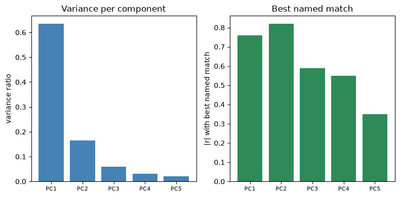
Left: fraction of embedding variance in each of the first five components. Right: absolute correlation of each component with its best-matching named measurement. The variance falls steadily; the named match is high for the first two components and low by the fifth.

The first two components have a named measurement that tracks them closely; by the fifth the best match explains little. So the names are worth having for the leading components and not beyond. The same idea applied to the embedding’s own dimensions, rather than to its components, would give pl.effect_sizes and tl.feature_sets something to key on again — borrowed rather than parsed, and honest as long as you say so.

Summary

• Test the unit that was randomized: aggregate cells to wells, then test. differential_features() refuses cell-level input.

• A rank test cannot call anything at two wells per treatment. diagnose_testing() says where your screen stands, and whether its p-values are calibrated.

• Blocking on plate refuses a layout where a treatment and its plate are the same variable.

• Read feature families rather than features. feature_signature() keeps the sign.

• An embedding has no feature names, but a named block measured on the same wells can lend its leading axes some.