Images and segmentations

Behind every profile there are images and segmentations. read_plate() reads a plate of them into a SpatialData object: fields of view as Images, the CellProfiler objects as Labels, and the cell-level measurements as a Table that annotates them.

jump_plate() is that call on two fields of view of well O09 of the JUMP plate BR00121438.

import matplotlib.pyplot as plt
import numpy as np
from spatialdata import get_pyramid_levels
from spatialdata.transformations import get_transformation

import mantispy as mt

sdata = mt.ds.jump_plate()
sdata

SpatialData object
├── Images
│     ├── 'BR00121438_O09_s1_image': DataTree[cyx] (8, 1080, 1080), (8, 540, 540), (8, 270, 270)
│     └── 'BR00121438_O09_s2_image': DataTree[cyx] (8, 1080, 1080), (8, 540, 540), (8, 270, 270)
├── Labels
│     ├── 'BR00121438_O09_s1_cells': DataArray[yx] (1080, 1080)
│     ├── 'BR00121438_O09_s1_cytoplasm': DataArray[yx] (1080, 1080)
│     ├── 'BR00121438_O09_s1_nuclei': DataArray[yx] (1080, 1080)
│     ├── 'BR00121438_O09_s2_cells': DataArray[yx] (1080, 1080)
│     ├── 'BR00121438_O09_s2_cytoplasm': DataArray[yx] (1080, 1080)
│     └── 'BR00121438_O09_s2_nuclei': DataArray[yx] (1080, 1080)
└── Tables
      └── 'cells': AnnData (284, 1989)
with coordinate systems:
    ▸ 'BR00121438', with elements:
        BR00121438_O09_s1_image (Images), BR00121438_O09_s2_image (Images), BR00121438_O09_s1_cells (Labels), BR00121438_O09_s1_cytoplasm (Labels), BR00121438_O09_s1_nuclei (Labels), BR00121438_O09_s2_cells (Labels), BR00121438_O09_s2_cytoplasm (Labels), BR00121438_O09_s2_nuclei (Labels)
    ▸ 'BR00121438_O09', with elements:
        BR00121438_O09_s1_image (Images), BR00121438_O09_s2_image (Images), BR00121438_O09_s1_cells (Labels), BR00121438_O09_s1_cytoplasm (Labels), BR00121438_O09_s1_nuclei (Labels), BR00121438_O09_s2_cells (Labels), BR00121438_O09_s2_cytoplasm (Labels), BR00121438_O09_s2_nuclei (Labels)
    ▸ 'BR00121438_O09_s1', with elements:
        BR00121438_O09_s1_image (Images), BR00121438_O09_s1_cells (Labels), BR00121438_O09_s1_cytoplasm (Labels), BR00121438_O09_s1_nuclei (Labels)
    ▸ 'BR00121438_O09_s2', with elements:
        BR00121438_O09_s2_image (Images), BR00121438_O09_s2_cells (Labels), BR00121438_O09_s2_cytoplasm (Labels), BR00121438_O09_s2_nuclei (Labels)

Coordinate systems

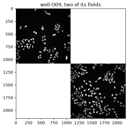
Every element sits in coordinate systems for its own field, its well and the plate. The well frame lays the fields of a well out where the microscope stage found them, with nothing resampled.

sorted(sdata.coordinate_systems)

['BR00121438', 'BR00121438_O09', 'BR00121438_O09_s1', 'BR00121438_O09_s2']

fig, ax = plt.subplots(figsize=(5, 5))
for image in sdata.images.values():
    offset = get_transformation(image, "BR00121438_O09").to_affine_matrix(input_axes=("y", "x"), output_axes=("y", "x"))
    y, x = offset[0, 2], offset[1, 2]
    dna = np.asarray(get_pyramid_levels(image, n=2).sel(c="DNA"))
    ax.imshow(dna, extent=(x, x + 1080, y + 1080, y), cmap="gray", vmax=np.percentile(dna, 99.5))
ax.set(xlim=(0, 2160), ylim=(2160, 0), title="well O09, two of its fields")
plt.show()

Images and labels

The image of a field carries one named channel per imaging channel, five fluorescent and three brightfield. The labels carry CellProfiler object numbers, so the rows of the cell table join straight onto them.

image = get_pyramid_levels(sdata["BR00121438_O09_s1_image"], n=0)
list(image.coords["c"].values)

[np.str_('Brightfield_L'),
 np.str_('Brightfield_H'),
 np.str_('Brightfield'),
 np.str_('RNA'),
 np.str_('Mito'),
 np.str_('ER'),
 np.str_('DNA'),
 np.str_('AGP')]

window = np.s_[300:600, 300:600]
fig, axes = plt.subplots(1, 4, figsize=(12, 3))
dna = np.asarray(image.sel(c="DNA"))[window]
axes[0].imshow(dna, cmap="gray", vmax=np.percentile(dna, 99.5))
axes[0].set_title("DNA")
for ax, name in zip(axes[1:], ("cells", "nuclei", "cytoplasm"), strict=True):
    ax.imshow(np.asarray(sdata[f"BR00121438_O09_s1_{name}"])[window], cmap="tab20", interpolation="nearest")
    ax.set_title(name)
for ax in axes:
    ax.set_axis_off()
plt.show()

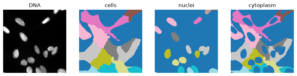
Cytoplasm is the cell mask minus the nucleus mask, as CellProfiler defines it.

The table

cells holds one row per segmented cell, with the cell’s own measurements as columns. It is an ordinary AnnData, and its var is annotated with what each feature name encodes, as read_profiles() annotates a profile read from disk.

cells = sdata.tables["cells"]
cells

AnnData object with n_obs × n_vars = 284 × 1989
    obs: 'Metadata_ImageNumber', 'Metadata_ObjectNumber', 'Metadata_Well', 'Metadata_Site', 'region'
    var: 'object', 'feature_group', 'feature', 'channel', 'scale', 'angle', 'gray_levels', 'radial_bin', 'params', 'is_feature'
    uns: 'mantispy', 'spatialdata_attrs'
    layers: None (.X)

cells.var.head()

	object	feature_group	feature	channel	scale	angle	gray_levels	radial_bin	params	is_feature
Cells_AreaShape_Area	Cells	AreaShape	Area	NaN	NaN	NaN	NaN	NaN	NaN	True
Cells_AreaShape_BoundingBoxArea	Cells	AreaShape	BoundingBoxArea	NaN	NaN	NaN	NaN	NaN	NaN	True
Cells_AreaShape_Compactness	Cells	AreaShape	Compactness	NaN	NaN	NaN	NaN	NaN	NaN	True
Cells_AreaShape_Eccentricity	Cells	AreaShape	Eccentricity	NaN	NaN	NaN	NaN	NaN	NaN	True
Cells_AreaShape_EquivalentDiameter	Cells	AreaShape	EquivalentDiameter	NaN	NaN	NaN	NaN	NaN	NaN	True

region names the Labels element each row annotates, and Metadata_ObjectNumber the label value inside it:

cells.obs[["region", "Metadata_ObjectNumber"]].head()

	region	Metadata_ObjectNumber
BR00121438_O09_s1_cells:1	BR00121438_O09_s1_cells	1
BR00121438_O09_s1_cells:2	BR00121438_O09_s1_cells	2
BR00121438_O09_s1_cells:3	BR00121438_O09_s1_cells	3
BR00121438_O09_s1_cells:4	BR00121438_O09_s1_cells	4
BR00121438_O09_s1_cells:5	BR00121438_O09_s1_cells	5

Reading a plate

A gallery source needs the accession directory, the batch and the plate barcode, which is what jump_plate() passes:

sdata = mt.io.read_plate(
    "cpg0016-jump/source_4",
    "BR00121438",
    batch="2021_04_26_Batch1",
    wells=["O09"],
)

wells defaults to every well whose images are present, so a partial download reads back as itself. The gallery publishes one-pixel object outlines rather than segmentation masks, so the Labels are reconstructed from them. A component is accepted only when exactly one object centroid falls in it and its area is close to the area CellProfiler measured. Rows whose object was not reconstructed are dropped, so every label stands for one object.

A plate straight out of a pipeline run needs only its folder:

sdata = mt.io.read_plate("run_export/Plate1")

Nothing is reconstructed on that path. The ExportForSpatialData module writes real label arrays, a per-cell table already joined across compartments, and a manifest in the table’s uns listing what it wrote.

Element names carry the plate barcode, so two plates concatenate without renaming, with spatialdata.concatenate([first, second], concatenate_tables=True).